I. Valtchanov, L. D. Spencer, C. Benson, J. Scott, R. Hopwood, N. Marchili, N. Hladczuk, E. T. Polehampton, N. Lu, G. Makiwa, D. A. Naylor, B. G. Gom, G. Noble, M. J. Griffin
HERSCHEL-HSC-TN-2321, Sep 2018 (revised May 2021)
The SPIRE Spectral Feature Finder Catalogue is the result of an automated run of the Spectral Feature Finder (FF). The FF is designed to extract significant spectral features from SPIRE FTS data products. These spectral features are only identified for High Resolution (HR) sparse or mapping observations, while for Low Resolution (LR) sparse or mapping observations the FF only provides the best fit continuum parameters. The FF engine iteratively searches for peaks over a set of signal-to-noise ratio (SNR) thresholds, either in the HR spectra of the central and off-axis detectors (sparse mode) or in each pixel (SPIRE Long Wavelength - SLW, and SPIRE Short Wavelength - SSW) of the two hyper-spectral cubes (mapping). At the end of each iteration, independently for each spectral band, the FF simultaneously fits the continuum and the features found. The residual of the fit is used for the next iteration. The final FF catalogue contains emission and absorption feature frequencies, and their respective SNR, for each observation; SNR is negative for absorption features. Line fluxes are not included as extracting reliable line flux from the FTS data is a complex process that requires careful evaluation and analysis of the associated spectra. Testing of the FF routine indicates that the FTS Spectral Feature Finder Catalogue is 100% complete for features above SNR=10, and 50-70% complete down to SNR=5. The full SPIRE Automated Feature Extraction Catalogue (SAFECAT) contains 167,525 features at |SNR| >= 5 from 641 sparse and 179 mapping observations.
Important notes:
The observations with FF products are listed in four coma-separated-value (.csv) files. These are available in the release and also in the FF legacy area topmost folder:
hrSparseObservations.csv: lists all the high resolution (HR) sparse-mode observations processed by the FF, including the HR part of H+LR observations. For each observation the file provides the following information: observation ID (obsid); source name (target); if the source is known to be featureless (knownFeatureless), and therefore no FF catalogue is provided; if the source has a significant spatial size (semiExtended or fully extended) or if it is pointLike (sourceExt); what data product was used for the FF (dataUsed), which can be the standard pipeline product spg from the Herschel Science Archive, a SPIRE Spectrometer calibration source Highly Processed Data Product calHpdp or data corrected for high background or foreground emission bgs; and if any bespokeTreatment was needed, such as special parameter settings.OffaxisObservations.csv: lists the 814 obsids included in the FF run for the off-axis detectors.hrMappingObservations.csv: lists the 180 HR mapping obsids included in the FF run.lrSparseObservations.csv: lists the 293 LR sparse obsids for which continuum parameters are provided.lrMappingObservations.csv: lists the 106 LR mapping obsids with continuum parameters.Section Individual FF catalogues and postcards provides links to all the individual obsid results.
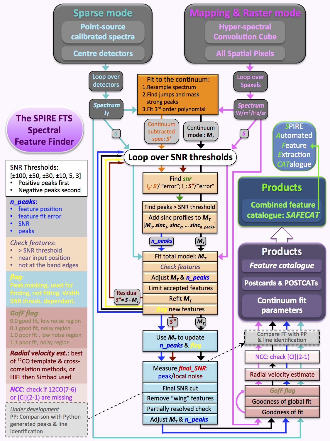
The Herschel SPIRE Spectral Feature Finder (FF) finding and fitting process is summarised by the flowchart shown in Fig. 1 and presented in full in paper I. This document briefly describes the main steps of the FF algorithm.
|
| Figure 1: flowchart for the FF processing (click the image to enlarge). |
The SPIRE FTS has two overlapping spectral bands: Spectrometer Short Wavelength, SSW (191-310 μm or 1568-944 GHz) and Spectrometer Long Wavelength, SLW (294-671 μm or 1018-447 GHz). They share an overlap region of 294-310 μm (1018-944 GHz). The primary input to the FF script is a single, per band spectrum, that has been extracted from one of the centre detectors (sparse mode) or a single spectrum from each of the two per band hyper-spectral cube spaxels (mapping).
Each feature found is fitted using a sinc-function (sin(x)/x) profile of fixed width, with the width set using the actual spectral resolution of the input data.
The following steps are carried out:
An input spectrum is resampled onto a coarser frequency grid (5 GHz for HR) and a "difference spectrum" is generated by subtracting the resampled spectrum from itself, after a shift of one frequency bin. No resampling is necessary for LR observations (1 GHz grid). The strong peaks correspond to "jumps" in the difference spectrum and are masked before a 3rd order polynomial is fitted (2nd order for LR). Neither the masking nor the peaks are carried forward into the main finding loop, only the polynomial model.
This is the only stage for LR observations (sparse or mapping) for which we only keep the derived continuum parameters.
We use the following SNR thresholds: +[100, 50, 30, 10, 5, 3] for emission and [-100, -50, -30] for absorption features.
For each threshold, the signal-to-noise ratio (SNR) spectrum is taken using the model subtracted residual and the spectrum dataset "error" column (for the first iteration the continuum model is subtracted).
Peaks are determined by merging all SNR data points that sit above the SNR threshold, within a 10 GHz width per peak.
Each new peak represents a potential new feature, so a sinc function is added to the total model (polynomial + sinc) per new peak found.
A global fit is performed using the input spectrum and total model, so all found and potential features, and the continuum, are simultaneously fitted.
For each SNR iteration, the resulting fitted sinc models for the potential features found are put through several reliability checks (e.g., checking their fitted position and looking for multiple peaks fitted to partially resolved features).
Features that are accepted as reliable have their fitted position limited to within a 2 GHz window before the global fit is repeated.
The resulting total model is carried forward to the next iteration, with the frequency either-side of each new feature masked by a SNR threshold dependent width, where no new features are permitted in any of the following finding iterations. The existing masking is updated to account for movement of already found features, noting that these have already had the position of their respective sinc models limited.
The final SNR is calculated using the fitted peaks and the total-model-subtracted residual spectrum as [fitted peak amplitude]/[local standard deviation].
Features with |SNR| >= 5 are carried forward to the final check - a search to discriminate unique features from fitting to the sinc wings of neighbouring significant features. The exception to this is an a posteriori check to preserve any [CI](2-1) detection, that falls within the wings of the strong 12CO(7-6) line (see step6).
To assess the distinction between false and true spectral features and to identify the likelihood of prospective spectral features being correctly identified, a goodness of fit metric has been developed that combines the goodness of fit for each individual feature found (GoF) with the Bayesian ratio (B10). GoF and B10 are used in conjunction to assign a flag to each identified spectral feature (FF flag). The relative weighting of the GoF and B10 in determining the spectral feature flags varies for different frequency regions within the SLW and SSW bands (e.g., the band edges are identified as suffering higher than average noise and thus are flagged using different criteria - see below).
The Feature Finder requires a goodness of fit metric that is not sensitive to the continuum or to line flux. Such a statistical metric, r, is calculated using a cross-correlation function between fitted feature and total model. r is not sensitive to the continuum, due to the subtraction of the local mean. r is also not sensitive to line flux, because of the division by the standard deviation of a given spectral region.
The Bayesian ratio B10, is defined as follows: B10 = logP(D|H1)−logP(D|H0), where P(D|H1) is the evidence for the total model H1 with the putative sinc-function feature in and P(D|H0) is the evidence for a model without it. As this is a probabilistic check, no assumption about the noise is made and therefore B10 is insensitive to systematic noise. B10 is complimentary to the r parameter identified above.
More details on the methods are provided in paper I.
0.0: good fit in lower noise region (FLAG_G_G)0.1: good fit in noisy region (FLAG_G_N)1.0: poor fit in lower noise region (FLAG_B_G)1.1: poor fit in noisy region (FLAG_B_N)The flagging criteria were chosen empirically.
r >= 0.64: good fitB10 <= -6 : good fitBoth criteria must be met for a "good fit", unless there are more than 35 features found in a given spectrum, in which case only GoF is considered, as B10 tends to return a null result.
The following regions are considered as noisy:
At the end of the Feature Finder (FF) process, for each high resolution (HR) observation, the radial velocity is estimated by searching for 12CO lines and the [NII] 205 µm atomic line, in the respective feature catalogue with identified 12CO taking priority over [NII]. In addition, a cross-correlation (XCOR) technique is applied using the feature catalogue and a template line catalogue, which includes most of the characteristic molecular and atomic lines in the far-infrared. For FF catalogues where few features have been found, XCOR includes an additional check with [NII] (for SSW) and 12CO(7-6) lines. These FF based estimates are compared to radial velocities from a collection by the HIFI team (Lisa Benamati, private communication).
More details on the methods are provided in paper I and paper II.
The following radial velocity related metadata are included in each FF catalogue:
RV - the radial velocity in the local standard of rest, in km/s. For sources at high redshift we use the convention that the radial velocity is equal to c*z, where c is the speed of light and z is the redshift: 1+z = νemitted/νobserved, where 'ν' is the frequency.RV_ERR - the error on the estimate, when available.RV_FLAG - the flag indicating the quality and the source of the radial velocity. Priority is given to the FF estimate when both XCOR and FF have comparable quality. The flags can be FF, FF?, XCOR, XCOR?, H?, S?, W17, or nan when unavailable (see descriptions in the list below). The question marks are used as a warning that the value is uncertain.
FF - confident estimate based on the Feature Finder 12CO or [NII] checks, also in agreement with the HIFI team collected radial velocities: either the difference is less than 20 km/s or the fractional difference is within 20% if the velocity estimate is > 100 km/s.FF? - good estimate based on the Feature Finder 12CO or [NII] checks, but either the difference with the HIFI provided value is larger than 20 km/s or the fractional difference is above 20% if the velocity estimate is > 100 km/s.XCOR- confident estimate based on the cross-correlation method and [NII], 12CO(7-6) checks, also in agreement with the HIFI team collected radial velocities: either the difference is less than 20 km/s or the fractional difference is within 20% if the velocity estimate is > 100 km/s.XCOR? - good estimate based on the cross-correlation method and [NII], 12CO(7-6) checks, but either the difference with the HIFI provided values is larger than 20 km/s or the fractional difference is above 20% if the velocity estimate is > 100 km/s.H? - when none of the FF or XCOR methods have reliable estimate then we use the HIFI provided value, if available. As the target names between HIFI and SPIRE may be different, as these are provided by the Herschel observers, we search the HIFI list for the nearest neighbour within 6 arcsec of the SPIRE central detector sky coordinates.S? - when there is no HIFI provided value and there are no good estimates by the FF and XCOR we use the radial velocity from Simbad. We search Simbad within 6 arcsec of the FTS central detector sky coordinates and assign the radial velocity from the nearest neighbour.W17 - for most extragalactic targets we search in Wilson et al (2017) for the nearest neighbour within 6 arcsec to the SPIRE central detector sky coordinates and assign the radial velocity from that work.nan - when neither internal method provide an estimate and no radial velocity information is available from Simbad, HIFI, or Wilson et al (2017).Warning: the radial velocities should be considered with caution, especially for sources with RV_FLAG having a ? or nan, as well as sources with very few lines.
The Neutral Carbon Check (NCC) is a focused check of the 12CO(7-6) and [CI](2-1) spectral region using the radial velocity from the previous step and the known rest frequency of these lines. If either one of these neighbouring features were missed by the main FF process, the NCC-identified missing feature is added to the final list of features found. If [CI](2-1) is detected by the nominal FF or the NCC, a similar search is performed for the [CI](1-0) line. Features detected or modified by the NCC can be identified as having the NCC_flag column in the FF products set to True. More details are provided in paper IV.
The main feature finder (FF) catalogue only considers the central detectors of the SLW and SSW detector arrays (SLWC3 and SSWD4) for sparsely sampled single-pointing observations. Most observations of this type are of sources that are point-like or have very little spatial extent in comparison to the SPIRE FTS beam Wu et al. (2013) (arXiv:1306.5780). During the development of the FF, we have identified 357 observations of semi-extended or fully extended sources that have a large spatial extent and are expected to have significant spectral information measured by the other 54 detectors that are off of the optical axis. These extended or semi-extended observations account for 41.1% of unique sparse observations. There is also a known potential for pointing errors in SPIRE FTS observations that can sometimes result in an observation straying as much as 1 arcminute from the requested pointing \citep{SPIREpointing} resulting in observations where the brightest emission is not seen by the central detector Sánchez-Portal et al. (2014) (arXiv:1405.3186).
The number of observations that are expected to have significant off-axis emission was estimated by comparing the integrated intensity across each off-axis detector within a given detector band to that of the respective central detector. 26.4% of sparse single-pointing observations have at least one off-axis SLW detector that is brighter than the SLWC3 detector in the respective observation and 25.1% have at least one off-axis SSW detector that is brighter than the respective SSWD4 detector.
The FF routine was applied to all HR sparsely sampled single pointing observations (1,025). Of these observations, 509 observations have detected features in the off-axis detectors yielding a total of 30,720 additional lines with an |SNR| >= 6.5. This off-axis |SNR| cutoff of 6.5 for emission features and 10 for absorption features is used to avoid spurious detections in these off-axis detectors that often have less intense spectra. Nominally a cutoff of SNR five is employed for emission features while an SNR cutoff of 10 is used for absorption features for the central detector spectra within the FF. This removal of spurious detections from off-axis detectors discards 36.3% of the features found in off-axis detectors.
An additional observation of the calibration source AFGL 4106 that is nominally excluded from the FF catalogue for central detectors is considered by the FF for off-axis detectors. This observation (ID 1342208380) suffers from an exceptionally large pointing error of ~24 arcseconds causing the source to be missed by the central SSWD4 detector and to be only partially observed by the SLWC3 detector. Treatment of the spectrum from the SLWC3 detector in this observation requires an extensive pointing offset correction which was deemed beyond the scope of the FF. The central source is not observed by any of the off-axis detectors but they do provide measurements of the surrounding emission from the galactic cirrus that do not require any such corrections. Although this observation was excluded from the nominal FF routine and resulting catalogue, it was included in the off-axis execution of the FF.
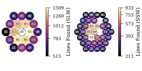 |
| Figure 2: The number of lines extracted by the feature finder shown for each off-axis detector. |
As one of the final steps in the feature finder (FF) routine, we attempt to determine the atomic/molecular transitions that correspond to the prominent FF spectral features. Through this work, SAFECAT not only provides to users the central frequency and SNR of significant spectral features but also provides information concerning likely molecular/atomic composition of sources.
In order to identify the atomic/molecular transitions that correspond to the spectral features extracted by the FF, these features are compared to a template line list of 307 atomic fine-structure and molecular features that are commonly found in astronomical sources at far-infrared wavelengths. The template is predominantly composed of spectral features from the CASSIS software Caux et al (2011), a free spectral analysis software designed to work with Herschel that can be accessed through the Herschel Interactive Processing environment (HIPE). A number of features that are also commonly found in SPIRE FTS spectra, such as the NII fine structure line, have been included in the template as well. The template makes use of the publicly available information contained in the following spectral databases: the NIST/Lovas Atomic/molecular Spectra Database Kramida et al (2018) Lovas (2004), the CDMS database Endres et al (2016), and the JPL sub-millimetre, millimetre and microwave spectral line catalogue Pickett et al (1998). The full list of the lines used in the template is detailed in Benson et al. These spectral features correspond to 15 different atomic/molecular species and encompass transitions from different isotopologues, ionization states, and vibrational bands.
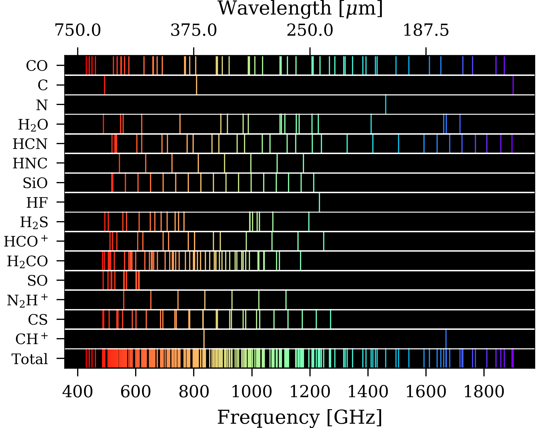 |
| Figure 3: Template lines shown in false colour representation. |
When multiple template features are matched to a single FF extracted line, all possible matches are reported in the catalogue and each is compared against the other identified lines to determine which of the possible atomic/molecular species has the most other identified lines. The most likely line of the multiple matches based on this criteria is then marked as the most plausible identification. If multiple species have the same number of identified lines, both features are marked as plausible and recorded.
The main FF catalogue does not report features with an |SNR| less than five in order to avoid the inclusion of spurious detections. There occur cases where an atomic or molecular species containing multiple lines in the SPIRE FTS band has some features detected near this limit with some actually falling below it. In the main execution of the FF these features would not be included in the catalogue. The line identification obtained by matching with the template provides a useful tool for extracting these low SNR lines that are not nominally reported by the FF. A check for low SNR features is done by iterating through the atoms/molecules identified in an observation looking for transitions that are expected to be found in the spectrum but are not contained in the FF results. This list of missing lines is then inserted into a second iteration of the FF routine as an initial central frequency guess for additional features during the final (and lowest) SNR threshold. Using this low SNR search routine we look for additional features down to |SNR|= 2 to add to the catalogue.
The line identification process and low SNR search routine are fully detailed in paper III.
Of lines with velocity estimates from sparsely sampled single pointing observations, 77.3% are successfully matched to the template and an additional 1,516 features are found by the low SNR search. Mapping observations provide a significantly larger data set of lines extracted by the FF than sparse observations and the majority of the observed sources are large extended emission regions. Of the lines from spaxels with reliable velocity estimates from mapping observations, 95.2% are successfully matched to the template by the line identification routine and an additional 370 lines are found by the low SNR search. The line identification routine successfully matches 93.1% of lines with velocity estimates from the spectra provided by off-axis detectors in sparsely sampled single-pointing observations with their corresponding atomic/molecular transitions. The low SNR search adds an additional 1,234 features from off-axis detectors in sparse observations.
For HR mapping observation the initial list of features for the subsequent FF iterations is provided by a python-based peak finder, applied on HR apodized spectra. This method provides better stability and avoids too many spurious features in noisy hyper-spectral cube pixels (spaxels).
Special calibration observations
Two observations, 1342227785 and 1342227778, were performed with special settings at two beam-steering mirror positions. In principle the pipeline successfully process them as mapping mode observations, and they are available in the Herschel Science Archive as spectral cubes with spatial coverage slightly better than sparse-mode and slightly worse than the intermediate sampling (4 BSM positions).
For the Feature Finder we used those observations as two separate sparse mode observations. In order to avoid files with the same name we changed their obsids to 1001342227785 (BSM position 1) and 2001342227785 (BSM position 2) for 1342227785, and to 1001342227778 and 2001342227778 for 1342227778. Hence their postcards, continuum parameters and feature catalogues will be available under these modified OBSIDs.
In order to include information from the off-axis detectors for these observations, they have also been processed by the mapping mode execution of the feature finder. These mappng products products use the standard obsids and can be found alongside other mapping products. SAFECAT reports only the lines from the mapping processed versions of these observations.
Highly Processed Data Products
Highly Processed Data Products (HPDPs) are available for the repeated observations of SPIRE Spectrometer calibration sources presented in Hopwood et al. (2015) (arXiv:1502.05717). These HPDPs are SPIRE spectra that have been corrected for pointing offset and, where necessary, for source extent or high background emission.
If an HPDP was used instead of the standard Herschel Science Archive product, this is reported under the metadata entry HPD_USED for the individual FF feature catalogues, and in the hpdp column of SAFECAT.
The Flag column (in the FF HR Sparse tables) indicates whether an HPDP was used, with an HPDP flag.
The HPDPs themselves can be accessed from the SPIRE-S calibration targets legacy data page.
HPDPs are also available for 22 SPIRE Spectrometer mapping observations that nominally super from one or more inidividual spectra have higher than expected spectral resolution. These 22 mapping observations were re-gridded without change to the majority of spatial pixels, although one or more pixels (of low quality) can be lost at the edge of the map. More information on these HPDPs is available on the ESA Herschel webpages.
The use of an HPDP regridded cube for a mapping observation instead of the cube from the standard Herscehl Science Archive Product is marked under the metadata entry HPD_USED for individual FF feature catalogues, and in the hpdp column in SAFECAT. HPDP flags for mapping products are as follows:
SLW - An SLW regrided cube was used in the FF execution.SSW - An SSW regrided cube was used in the FF execution.Both - Regridded cubes for both SLW and SSW cubes were used in the FF execution.None - No regridded cubes were used in the FF execution.The HPDPs themselves can be accessed from the Herschel Legacy HPDP repository area.
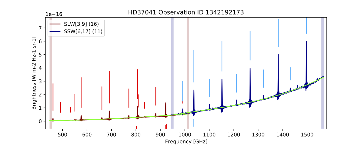
The observations 1342192173, 1342192174, 1342192175, 1342204898, 1342204920, 1342214827, 1342214841, 1342214846, and 1342228703 all received special treatment and processing time by the FF team since the nominal FF script did not provide satisfactory results. Observational products and SAFECAT results for these obsids reflect the results of the modified FF routine operating on the standard non-HPDP non-regridded spectral cubes. The FF results from a single SSW pixel and its corresponding SLW pixel from 1342192173 are shown below as they appear in FF products and as processed by the nominal FF script. Whether regridded cubes are used or not, it is expected that results from a careful case-by-case line fitting will result in negligible differences. The differences between the figures below are a result of the extra care afforded to the observation by the FF rather than the use of the regridded HPDP.
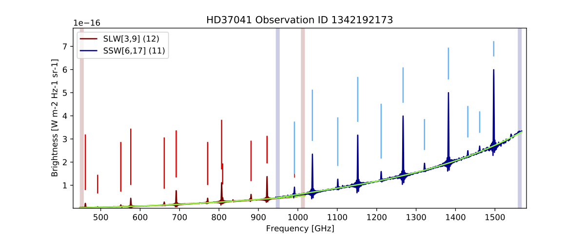 |
| Figure 4: FF results from a pair of matching pixels from observation 1342192173. These results were produced by a modified version of the public FF script and do not make use of the re-gridded SSW available for this observation. This product reflects the results used in FF products for this observation. |
 |
| Figure 5: FF results from a pair of matching pixels from observation 1342192173. These results were produced by the standard FF script operating on the observation with its re-gridded SSW cube. Note that the routine has incorrectly fit the CO(8-7) transition. |
Background Subtracted (BGS) Spectra
bgs for the individual FF feature catalogues, and in the bgs column of SAFECAT.Flag column (in the FF HR Sparse tables indicates whether BGS data was used, with a BGS flag.If, for a particular observation, non-default FF parameters were used or bespoke treatment was applied, this is indicated with a "1" in the bespokeTreatment column of hrSparseObservations.csv, which lists all HR observations for which there is a set of FF products.
Fewer negative SNR thresholds
By default, the FF iterates over a number of SNR thresholds when looking for peaks: +[100, 50, 30, 10, 5, 3] followed by [-100, -50, -30, -10] for absorption features. For one particularly spectral rich observation (OBSID: 1342210847), if the default set of negative SNR thresholds is used, there are so many features found that there are not enough unmasked data points available for the final SNR estimates, and thus many features are discarded. This loss of features is prevented by omitting the -30 and -10 SNR threshold iterations.
Final SNR estimate
To optimise the final SNR estimate, the FF stipulates that the number of unmasked data points in the local region used to calculate the residual standard deviation must be at least 17 (5 GHz). If this condition is not met, then the local region around the fitted peak is widened.
For the observations of two spectral rich sources (OBSIDs: 1342192834 and 1342197466) this condition is never matched for the majority of the features found; using the default FF settings, the majority of features are discarded. For these two cases, no minimum is set for the number of data points required for the the final SNR estimate to go ahead.
Features added by hand
During the FF SNR threshold iterations, the SNR is taken using the spectral dataset "error" column. For a handful of observations this can lead to no significant SNR peak at the position of significant spectral peaks and the corresponding features are therefore never found by the FF, regardless of how low the SNR threshold drops.
A handful of missing significant features were added at the appropriate SNR threshold during the FF process for six observations: OBSIDs 1342197466, 1342248242, 1342216879, 1342197466, 1342193670 and 1342210847.
With 1041 HR sparse observations, 868 are input to the FF line search (excluded targets include restricted (i.e., not public) observations, solar system objects (i.e., planets and asteroids), and dark-sky observations) and have continuum fit parameters reported in SAFECAT. Of the 643 HR sparse observations with spectral features identified by the FF, 287 are included only in the point-source calibrated data and 356 have entries in both the point and extended calibration FF data.
The Feature Finder produces feature catalogues for all SPIRE Spectrometer HR sparse and mapping mode observations, unless these are of known featureless sources (e.g. the asteroids Vesta, Ceres) or the target is not included in the FF list of observations (e.g. dark sky and sources with well developed models, including Uranus, Neptune and Mars). Failed observations and calibration observations with unusual settings are also omitted.
The Feature Finder catalogues are available as FITS files with the catalogue and its metadata in the first Header Data Unit (HDU).
The sparse mode catalogue table contains the following columns:
frequency - the measured frequency, in GHz, of features found with absolute(SNR) > 5 (noting that negative SNR corresponds to absorption features)frequencyError - the error on the measured frequency, also in GHzSNR - the SNR measured using the fitted peak and the local noise in the residual spectrum (after the total fitted model has been subtracted)detector - which detector the feature was found in (SLWC3 or SSWD4 for sparse-mode observations)featureFlag - a flag to show if the fit is considered good or poor and if the feature is in a high noise or lower noise region of the spectrum. The flags are explained in more detail in section FF feature flags.NCC_flag - a flag, which if true, indicates that a feature was detected or modified by the NCC.Note #1: the frequency axis of all SPIRE spectra, as well as those from the other Herschel spectrometers, are provided in the kinematic Local Standard of Rest (LSRk). Consequently the measured frequencies in the FF are also in the same LSRk reference frame.
Note #2: no consolidation of features in the overlap region (944-1018 GHz) has been performed. Therefore the same feature may be present for both central detectors for the same observation.
The mapping mode catalogue table contains the following additional columns:
row - the cube row pixel where the feature is foundcolumn - the cube column pixelra - the RA (in degrees) for the corresponding pixel where the feature is founddec - the Declination (in degrees) for the corresponding pixel where the feature is foundarray - instead of the detector name, this column provides the FTS array name, can be SSW or SLW.velocity - the radial velocity estimate of the pixel in which the feature was detected.velErr - the associated error in the radial velocity estimate.vFlag - the velocity flag associated with the radial velocity estimate. Universally FF?, or nan if no valid velocity was obtained.Note: the SSW and SLW hyper-spectral cubes have different world-coordinate-systems (WCS), their pixel size and centres are not matched, i.e., row and column are array dependent. This is clearly evident within the SLW and SSW maps presented in the mapping postcards (see Fig. 5).
In addition to the catalogue table, the mapping FITS file contains 5 more HDU extensions: velocity, velocityError, vFlags, nLines, and arrays. In deriving radial velocity estimates for mapping observations, features detected within the SLW map were projected into an SSW equivalent grid. The number of lines within each pixel of the synthesized map and which maps these lines originally came from (L for SLW and S for SSW) is indicated in the nLines and arrays HDU extensions, respectively. The velocity, velocityError, and vFlags extensions indicate the estimated radial velocity, velocity error, and associated velocity flag of the pixels in the synthesized map. The vFlags HDU uses the notation (N,M), where N indicates the number of 12CO candidate features used to derive the velocity estimate, and M indicates the number of matches each candidate feature has with the characteristic difference array of the 12CO ladder (see paper II, for more details). The closer these values are to 10, the more reliable the velocity estimate is expected to be. Velocity estimates based on the [NII] feature are denoted by NII,1.
The catalogue FITS extension metadata contain the following information:
FLAG_* - feature flag definitions, see section FF feature flags;OBS_ID), the source name as given by the observer (OBJECT); the commanded source coordinates RA_NOM and DEC_NOM, the operational day (ODNUMBER) when the source was observed; the resolution (COMBRES); the bolometer detectors bias (BIASMODE); and the map sampling (MAPSAMPL);MIN_SNR equal to 5) and the region avoided at the ends of the frequency bands (EDGE_MASK equal to 10 GHz);MAX_CONT;N_SSW and N_SLW;RV), the error associated with that estimate (RV_ERR) and a radial velocity flag (RV_FLAG); these are described in section Source radial velocity estimate.S_EXTENT), as classified from assessing the quality of the spectra in comparison to any associated PACS photometer maps (pointLike, semiExtended or extended). This keyword is not available for mapping mode (where extended source calibration is used by default);CAL_TYPE, can be pointSource or extended) and units of the data (FLXUNIT which can be Jy or W/m2/Hz/sr);HPD_USED = True|False) or spectra that have been corrected for high background or foreground emission (BGS_USED = True|False) were used. More information on the HPDPs used by the FF can be found on the SPIRE-S calibration targets legacy page. The background subtracted data used for the FF can be found in the Herschel legacy area. These are only present for sparse mode; mapping observations make use of a modified HPD_USED flag, with possible values of SLW|SSW|Both|None. More information concerning mapping mode HPDPs can also be found in the in the Herschel legacy area.The SAFECAT contains all the features found from the catalogues per observation for SPIRE Spectrometer HR sparse and mapping observations. SAFECAT is intended as an archive mining tool that can be searched by frequency, position, etc., to provide all SPIRE Spectrometer observations with significant features that match the search criteria.
SAFECAT_v3 contains results from the central and off-axis detectors from sparse observations and results from mapping observations, and contains the following columns:
obsid: the observation ID;opDay: the operation day for the observation;frequency, frequencyError: the fitted feature position in GHz and the error on this measurement, in LSRk frame.SNR: the signal-to-noise ratio of fitted peak to local noise in the full residual;array the bolometer detector array name where the feature was detected in. For sparse mode SSW and SLW are used to denote the central detectors SSWD4 and SLWC3 respectively. row, column: the (row,column) pixel for mapping mode or (-1,-1) for sparse;ra, dec: the RA and Dec (J2000.0) of the central detectors for sparse mode or the RA and Dec of the corresponding (row,column) pixel for mapping;featureFlag: the feature flag, as explained above;velocity, velocityError: the source radial velocity and its error, in km/s;velFlag: the radial velocity flag following subsection Radial velocity metadata and flags.extent: whether the source is pointLike, semiExtended or extended, categorised as explained above. It is always extended for mapping;calibration: which calibration was used. It is always extended for mapping, while for sparse could be either extended or pointSource.sampling: the spatial sampling of the observations, can be sparse, intermediate or full.bgs: whether a background subtracted data product was used by the Feature Finder;hpdp: whether a highly processed data product was used by the Feature Finder;NccFlag - identifies features detected or modified by the NCC. In total, 162 obsid and 4781 features have this flag on.velocityCorrFreq: the frequency of the fitted feature shifted to the "rest frame" based upon the source radial velocity.templateFrequency: the rest frequency of the template line that has been matched to the fitted feature through the line identification routine.species: the atomic or molecular species corresponding to the template line that has been matched to the fitted feature.transition: the transitional quantum numbers corresponding to the template line that has been matched to the fitted feature.comment: a comment string to differentiate between multiple template matched to a single fitted feature. Multiple template matched to a single FF extracted feature are marked with a character from a-z and the most likely candidate according to the line identification routine is marked with an underscore character. E.g., a comment of 'b_' denotes the second template line that has been matched to the fitted feature which is considered to be the most likely candidate. A '!' character in the comment column denotes a line that has been added by the low SNR search.'The metadata provides the feature flag definitions; the minimum SNR cut applied (5); the frequency range avoided at the ends of the bands (10 GHz); and lists two special calibration observations and the unique IDs assigned for the purpose of SAFECAT only, as they consist of two sparse pointings in one observations.
Molecular species follow a convention where the number of a particular atom (typically denoted as a subscript) follows the atom it pertains to. E.g., water is denoted H2O. Isotope numbers (typically denoted as superscripts) follow the atom they pertain to and are separated by two - characters. E.g., the 13C18O carbon monoxide isotope is denoted C-13-O-18. Occasionally a vibrational band is also denoted sometimes as a range. E.g., CS, v=0-4 indicates that the transition arises from the Carbon Sulphide molecule in a vibrational band between v equal to 0 and 4.
The conventions for quantum numbers are fully discussed in paper III. Transitions are separated by an underscore character (_) and numbers most commonly represent rotational states. Fine structure lines use a -> to separate the quantum numbers in a transition.
When multiple template lines are matched to a single FF extracted feature, multiple rows are created in SAFECAT. The nominal FF information for the fitted feature is repeated and the different template lines are assigned respective comment characters.
If a FF feature has no match in the template the rest frequency and template columns are given not a number (NaN) or null values and the species and quantum number columns receive -- characters. Such cases are marked by a noID comment.
The SPIRE FTS instrumental line shape (ILS) is essentially a sinc function (sin(x)/x). The sinc-like wings of each feature introduce ringing, which, although decreasing in amplitude, does extend over the whole frequency range. Therefore, to gain a good fit to the continuum, this sinc ILS should be simultaneously fitted with the main spectral features.
During the Feature Finder finding and fitting process, a 3rd order polynomial (2nd order for LR) is fitted to the continuum per band spectrum, in conjunction with sinc functions for each feature found. The resulting continuum fit may be hard to precisely recreate, unless a similar procedure is carried out. Therefore the best fit polynomial parameters for the continuum are provided with the other Feature Finder products.
The parameters are of the form:
p0 + p1*v + p2*v^2 + p3*v^3 (or p0 + p1*v + p2*v^2 for LR),
where v is the frequency.
The frequency ranges for the SPIRE FTS, used in the continuum calculations, are [446.99, 1017.80] GHz for SLW and [944.05, 1567.91] GHz for SSW.
For a given observation, the associated fittedContinuumParameters FITS file contains a table in the first HDU with the parameters for each detector that has been through the Feature Finder algorithm: the centre detectors for sparse observations, and each pixel for mapping observations.
For sparse mode the fitted polynomial is also provided as a Herschel spectrum dataset, with the best fit parameters reported in the metadata. The dataset is stored in a FITS file with each detector in a separate HDU, identified by the detector name, e.g. hdu["SSWD4"] will contain the continuum spectrum for the central detector of the SSW bolometer array. The frequency grid in these spectra is the same as the input ones.
The Feature Finder results are visually summarised per observation in a “postcard”. Each postcard compares the input spectra for the centre detectors, the best fit to the continuum, and includes vertical ticks representing the features found (with these arbitrarily scaled by the signal-to-noise). Fig. 2 provides a few examples of postcards.
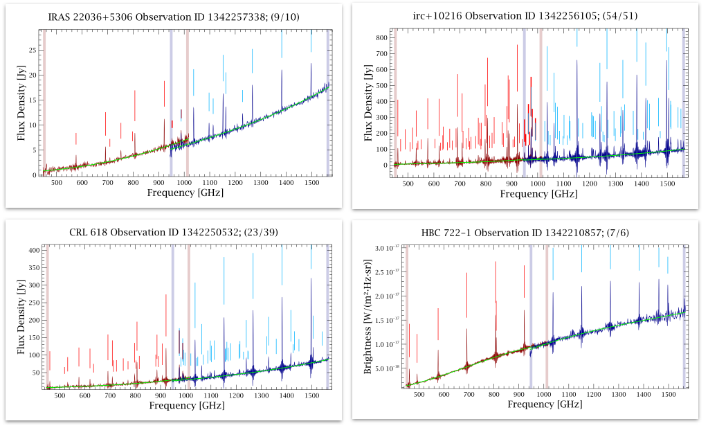 |
| Figure 6: Example postcards for 4 different observations, 3 are point-sources (the vertical axis unit is in Jy), while the bottom right one is extended (the unit is in W/m2/Hz/sr). The original spectra are shown in blue (SSW) and red (SLW), the best-fit continua are shown in green, the features are indicated with short vertical ticks, above the feature (emission) or below (absorption). The semi-transparent vertical thick bars indicate the regions where the calibration is uncertain - the noisy regions where the features are flagged (see FF feature flags). |
By default, the Feature Finder operates on point-source calibrated data, which has flux density units of Jy. For sources with some spatial extent there is also a postcard for the extended-source calibrated data, which has surface brightness units of W/m2/Hz/sr. Both postcards for such sources are included in the product pages, accessible via the tables at the end of the Feature Finder Release Note.
If an observation of interest is of a partially or fully extended source, it is advisable to visually check both sets of FF results. These are available in one combined postcard in folder HRpointProducts/HRdoublePanelPostcards, an example is shown in Fig. 3.
 |
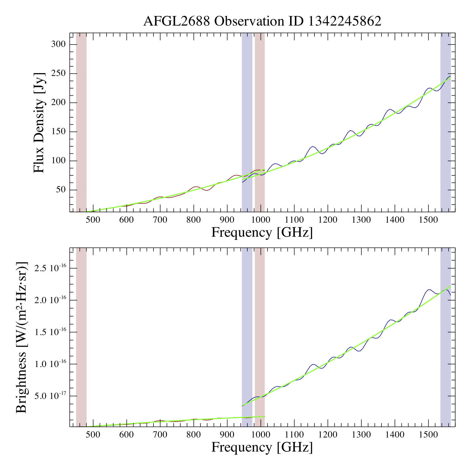
| Figure 7: Example postcards for one `OBSID` and the results of the FF run on both point-source (top) and extended-source (bottom) calibrated spectra. In this particular example the source is fully extended, as can be inferred by the good match of the two bands (blue: SSW and red: SLW) in the overlap area for extended-source calibrated spectra. This `OBSID` is marked `extended` in hrObservations.csv) file. |
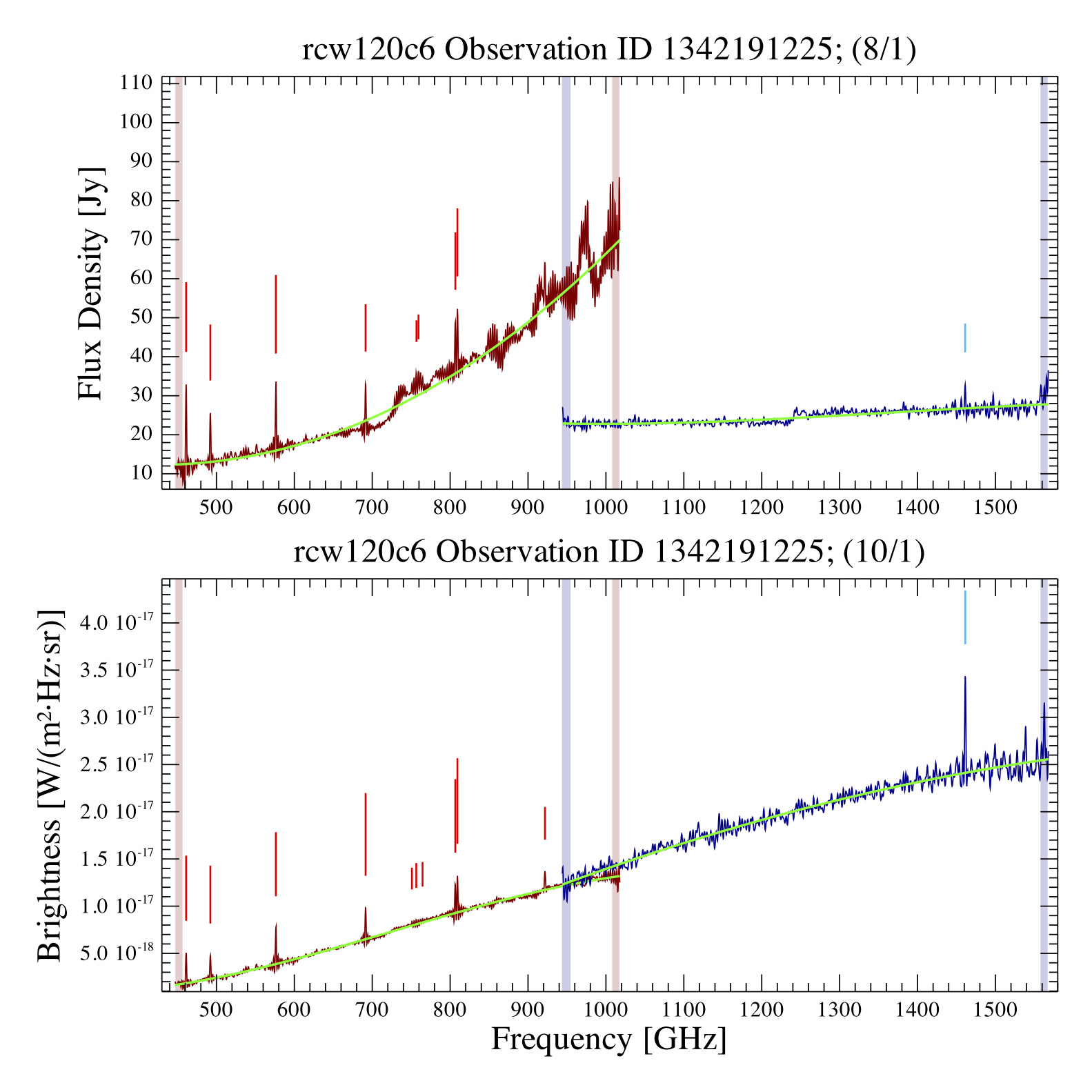
For LR observations no features are provided, as LR was primarily aimed at providing a measurement of the continuum and there are few features found in these observations. However, two postcards are provided for LR, as shown in Fig. 4. Many targets are semi-extended in nature and simply by comparing the postcards it may be possible to gauge which calibration scheme is more appropriate (or if there is a problem that may require further processing to correct for partial extent). Visual inspection should evaluate the continuity of the SLW/SSW spectra within the spectral overlap region.
 |
| Figure 8: Example postcard for one LR observation, both point-like (top) and extended versions (bottom) are provided. The good match of SSW and SLW in the overlap area in the top panel is an indication that the source is point-like. |
The Feature Finder mapping results are also visually summarised per observation in a “postcard”. Each postcard is comprised of a 2x3 array of figures illustrating various aspects of the observation.
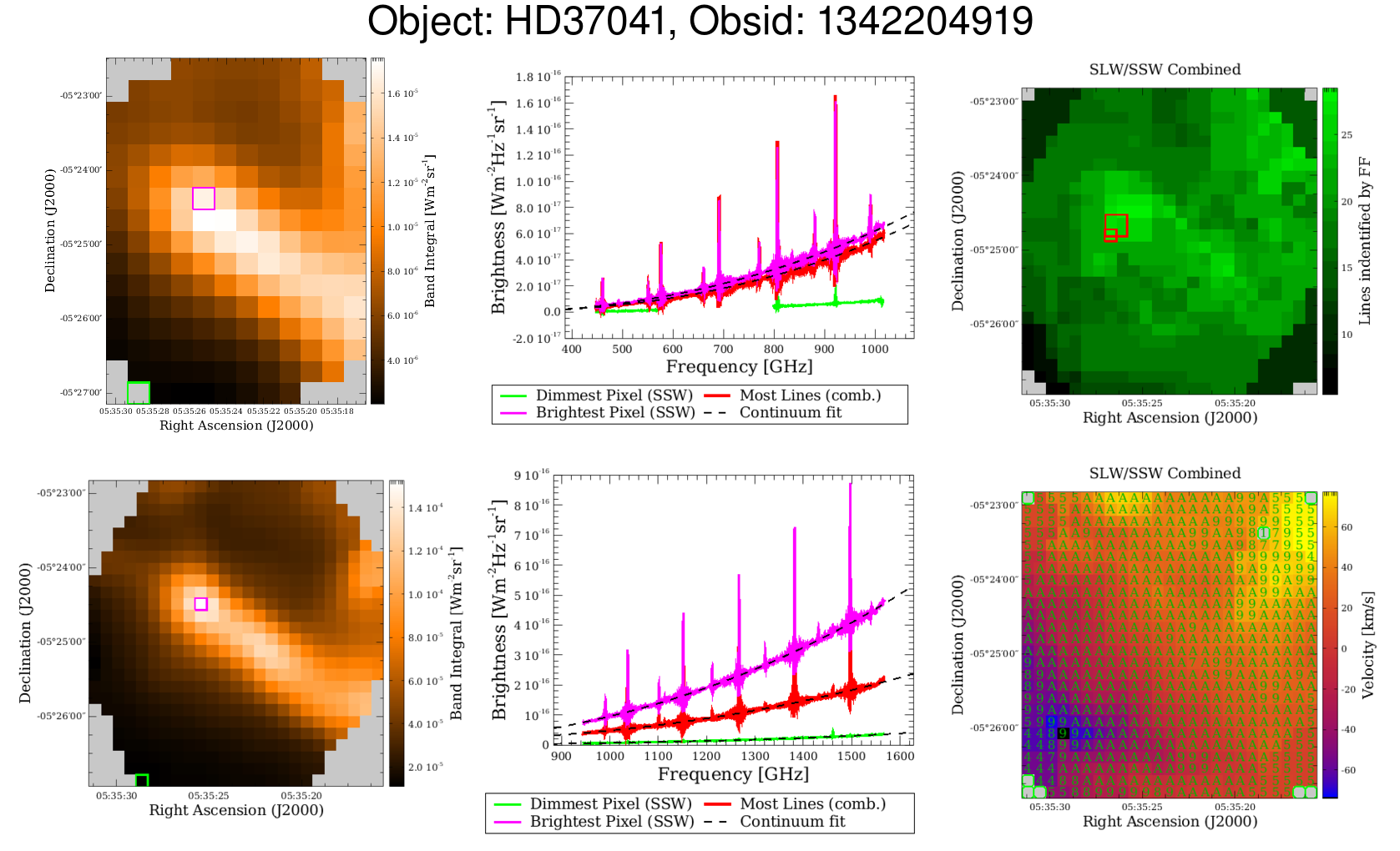 |
| Figure 9: Example postcard for one mapping observation. |
The left column illustrates the integrated flux associated with each band, with SLW on top and SSW on the bottom. Note the difference in pixel sizes for the SLW and SSW maps. Each of the integrated flux maps in the left column have two pixels identified for each band with coloured box outlines. For the SSW array, these correspond to the dimmest and brightest pixels within the map. For the SLW array these pixels correspond to the closest SLW pixels to the identified brightest and dimmest pixels for the SSW array.
The central column presents the spectra corresponding to the flagged pixels in the flux maps (brightest and dimmest integrated flux pixels for SSW, closet match for the SLW array) with SLW on top and SSW on the bottom. Also shown in the central column is the spectrum corresponding to the pixel with the most spectral features identified by the FF, again with SLW on top and SSW on the bottom.
The upper right figure is a map of the number of lines identified by the FF in both the SLW and SSW arrays combined (equivalent to the nLines HDU extension in the mapping products). This figure also has the pixel regions associated with the most lines in the SLW and SSW arrays identified with coloured box outlines. As the SLW pixels are larger than the SSW pixels, the SLW lines may be counted in multiple SSW pixels within this FF histogram map.
The lower right figure presents the FF radial velocities provided by the radial velocity routine (equivalent to the velocity HDU extension in the mapping products). The results are shown on SSW pixels, with the pixel colour indicating the velocity (colour-bar on the side), and a code within each SSW pixel indicating the quality of the radial velocity. Within the radial velocity map, a marker of A means all of the expected CO lines contributed to the radial velocity estimate, N means that the [NII] nitrogen spectral feature was used, and a number indicates the number of CO lines used in the radial velocity estimate (less than all of the expected lines were identified).
The header of the mapping postcard indicates the target name, as provided by the observer, and the observation number (OBSID). Pixels outlined in green on the velocity map highlight pixels where the feature finder did find spectral features but the radial velocity routine did not provide an accurate velocity estimate.
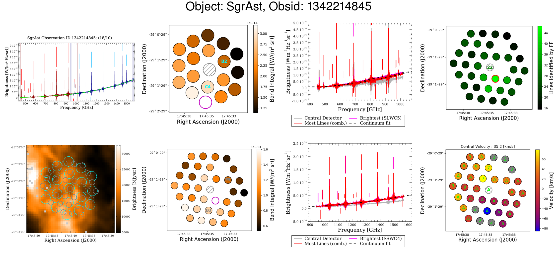 |
| Figure 10: Example off-axis postcard for one sparse observation. |
The postcards developed to highlight off-axis spectral content extend the previously developed sparse postcards for central detectors and parallel the mapping postcards as much as possible. The postcards are composed of 8 panels. The first of the four columns of the postcard displays the sparse postcard that was generated in the nominal FF process (top) and the SPIRE FTS footprint over the SPIRE photometer short-wave (PSW) map (bottom). For the photometer map, the figure itself is centred on the requested pointing of the observation and cropped to a 4 arcminute square. The colourbar of the photometer map is scaled to reflect the image content and empty pixels which are assigned a not-a-number (NaN) value are coloured in grey. The SPIRE footprint is shown with its actual pointing for each detector, the SLW array is outlined in cyan and the SSW array is outlined in grey. The circles represent the FWHM of the detector beam at the centre of the band corresponding to each array. In cases where no SPIRE photometer map is available for the pointing of the FTS observation, a stock image stating that no photometer map was found is shown instead. There are 97 SPIRE FTS observations for which no photometer map was observed.
The second column contains the footprint of each detector array on sky (SLW top, SSW bottom). Each off-axis detector is coloured based on the integrated intensity across their entire band for the given observation, with the extended source calibrated spectrum used for this calculation. The central detector is not included in the determination of the colourbar dynamic ranges and it is marked by the grey hashed-out circle to illustrate this. In order to determine the orientation of the detector arrays, the SLWC3 and SLWB2 detectors are labelled in cyan while the overlapping SSW detectors, SSWB3 and SSWE5, are marked in grey. Note the two dead detectors in the SSW array which also help in determining the orientation of the FTS on-sky. The brightest detector from each array is outlined in magenta. This intensity map of the FTS footprint with the photometer map provides information about the structure of the source which should correspond to the spectral content of off-axis detectors.
The third column presents a few spectra of interest from the SLW (top) and the SSW arrays (bottom). The spectra from the brightest off-axis detectors are plotted in magenta (based on the band integrated intensity and marked in the corresponding panels to the left) and the spectra from the detectors with the most lines are plotted in red (marked in the upper panel to the right). The spectrum from the central pixel is also plotted in the figure background, in grey, and intentionally without influencing the vertical axis limits. The central spectrum is only provided for comparison and is better viewed in the central detector postcard (top left panel). Again the extended source calibration spectra are chosen for these plots. The spectra with the largest number of lines is determined by combining the lines extracted from each SSW spectrum with those from its nearest neighbouring SLW spectrum, the number of features is then determined as the total number of features from both. As is the case for central detector postcards, the lines extracted by the FF are marked by vertical sticks with lengths proportional to the SNR of the feature. Emission features are marked above the spectra while absorption features are marked below.
The fourth and final column contains the number of lines extracted by the FF (top) and the radial velocity estimates (bottom) from off-axis detectors. In each case, the lines extracted from the SSW detectors are paired to the nearest SLW detector and used for velocity estimates and the total number of lines displayed in each SSW detector. The SSW off-axis detector with the most number of lines found by the FF is outlined in red. The number of spectral features found by the FF for the central detector is written in green on the central detector. The velocity estimates are obtained from the CO velocity estimate routine and follow similar annotations to those in mapping postcards. The green numbers mark the number of CO features used in the velocity estimate with the character 'A' denoting that all 10 in-band CO features are used. When the NII feature is used for the velocity estimate an 'N' character is used instead. Detectors for which no reliable velocity estimate can be obtained by the CO method are coloured in grey. The radial velocity estimate from the central pixel is also shown in the title of the velocity panel and the radial velocity flag is printed in green over the central pixel.
Each sparsely sampled single-pointing observation has a feature finder product which contains the line fitting results for each off-axis detector. This product contains similar data columns and meta data as in the nominal sparse observation products for the central detectors and also contains a table with the velocity information for off-axis detectors. Off-axis detectors employ both the CO velocity method as well as the cross-correlation method (see paper II) for detectors where the CO routine is unable to determine a reliable velocity estimate. Off-axis velocities employ the same flag convention as for mapping observations and includes a 'XCORR?' flag for velocities determined by the cross-correlation method. Velocities determined by the NII feature are appropriately flagged. When no reliable velocity estimate is obtained for an off-axis detector, the table simply reports a row of NaN values and a '--' string as a flag.
The FF products are available as Highly Processed Data Products (HPDP) in the Herschel legacy area and also in the Herschel Science Archive (HSA).
The HSA is providing access to the individual FF products linked to a particular observation ID, while the HPDP gives access to all products within a web browser.
All products, including off-axis processing and line identifications, are combined in a single tar.gz file: FF_v3.tar.gz.
At the top level, there are a number of CSV files, which are described in section Observations.
The folders and their content are described below:
HRextProducts: contains FF products for
extended-source calibrated data of HR sparse observations, but only for
sources categorised as extended in hrSparseObservations.csv. All products based on running the FF on extended source calibrated spectra have _ext in the name.
HRpointProducts: contains the products for
all HR sparse observations processed with the FF, using the point-source
calibrated spectra. All products based on running the FF on point-source calibrated spectra have _pnt in the name.
HRextProducts-offaxis: contains the products for
all HR sparse observations off-axis detectors, processed with the FF. The products have _offAx in the name.
Each folder have sub-directories containing the FF postcards (postcards),
the best fit continuum parameters (continuumParameters), the continuum in a spectral dataset (continuumSpectrum, not available for offaxis products), and the FF feature catalogues (featureCatalogues). The files in these subfolders are per OBSID. The HRpointProducts folder also contains a sub-folder HRdoublePanelPostcards with the combined postcards for the FF results for both point and extended calibrated spectra.
HRmapping contains the products for all HR mapping observations. There are sub-directories containing the FF postcards (postcards),
the best fit continuum parameters (continuumParameters) and the FF feature catalogues (featureCatalogues). Note that only the convolution projection hyper-spectral cubes were used in the FF run.
LRproducts is the topmost folder for all low resolution (LR) FF
products. There are subfolders for point-source (LRpoint), extended-source calibrated spectra (LRext) and mapping observations (LRmap). These
also include the LR part of H+LR observations. Each of these sub-folders contain sub-sub folders with the best fit continuum parameters (continuumParameters) and FF postcards (postcards). The LR mapping products have a further subdivision for hyper-spectral cubes with the convolution projection (CP) and "Naive" projection.
All LR products (postcards or continuum parameters) based on point-source calibrated spectra have _pnt_lr in the filename. Similarly for extended-source calibrated spectra the filename will contain _ext_lr.
For LR mapping, the products will have _cp or _naive in the filename, depending on which hyper-spectral cube version was used: the convolution projection or naive.
The FF results, with some additional information, are also tabulated in a number of HTML pages, linked in the tables below. Each table provides links to the FF product tables in the left-hand column. The observations included on each page is given in the middle column, with the corresponding operational days in the right-hand column.
| Go to page | Observations covered | Operational days |
|---|---|---|
| HR sparse-mode FF products | HR Sparse Page 1 | 1342187893 — 1342212341 | 209 — 602 |
| HR Sparse Page 2 | 1342212342 — 1342231985 | 602 — 908 |
| HR Sparse Page 3 | 1342231986 — 1342247763 | 908 — 1151 |
| HR Sparse Page 4 | 1342247764 — 1342258698 | 1151 — 1335 |
| HR Sparse Page 5 | 1342258699 — 1342270195 | 1335 — 1434 |
| HR mapping-mode FF products | ||
| HR Mapping Page 01 | 1342192173 — 1342245117 | 302 — 1079 |
| HR Mapping Page 02 | 1342245083 — 1342270045 | 1080 — 1433 |
| LR sparse-mode FF products | ||
| LR Sparse Page 1 | 1342188674 — 1342248229 | 227 — 1160 |
| LR Sparse Page 2 | 1342248245 — 1342257934 | 1160 — 1326 |
| LR Sparse Page 3 | 1342259570 — 1342270194 | 1340 — 1434 |
| LR intermediate and fully sampled mapping mode FF products | LR Mapping Page 1 | 1342192179 — 1342262926 | 302 — 1362 |
| LR Mapping Page 2 | 1342262927 — 1342270038 | 1362 — 1433 |
Ivan Valtchanov, Locke Spenser, Chris Benson, Jeremy Scott Revised May 2021.