2.5 Quality assessment and validation
Author(s): Uli Bastian
2.5.1 Overview
Author(s): Uli Bastian
An extensive continuous assessment and validation was performed on all astrometric and photometric pre-processing products, as well as on the telemetry input data entering the pre-processing steps.
In this section, the highest emphasis is given to the monitoring of the daily pre-processing (IDT) and to the monitoring of the sole cyclic pre-processing step (namely the IDU crossmatch) for Gaia DR1. These two processes produced output which directly entered the generation of the astronomical contents of the Gaia DR1.
The other three relevant quality assessment and validation processes — namely the First Look (FL), the AVU Astrometric Instrument Model (AIM) and the AVU treatment of the Basic-Angle Monitoring data (AVU–BAM) are described much more briefly and just for completeness. They contributed to the quality of the Gaia DR1 — e.g. by finding on-ground processing defects and disturbing on-board phenomena, so that those defects and problems could be mitigated as far as possible. But no data products from FL, AIM and AVU–BAM directly contribute to the input data generating the astrometric and photometric source parameters in Gaia DR1.
2.5.2 Monitoring of daily pre-processing
Author(s): Jordi Portell, Michael Biermann, Deborah Busonero, Alberto Riva
Daily pre-processing results are closely monitored both by IDT and FL systems. Monitoring in IDT is relatively simple, being composed of counters, statistics, histograms and the like. The advantage is that IDT must process all of the science data received from the spacecraft.
On the other hand, FL only handles a subset of data — mainly detections brighter than and some fainter detections arriving promptly enough from the spacecraft, but these FL checks are more exhaustive. Some simple statistics and histograms are also determined, but these include automatic alarms to detect unexpected deviations in any of the many output fields. Also, FL runs complex algorithms to determine one-day calibrations (including a first astrometric solution), which not only serve as updated calibrations for IDT, but also provide details on variations and trends in the instrumentation and even in IDT processing outputs in themselves.
IDT Monitoring and Validation (IDV)
IDT monitoring is mainly done through a web interface which called WebMon, which acts as a front end to the many statistics and plots generated by the system on-the-fly. That is, diagnostics are continuously compiled in IDT (mainly histograms) on the outputs generated by the system. Most of these diagnostics are computed over typically one day of data. Some of the most remarkable ones are the following:
-
•
Performance monitor:
-
–
Plots with the OBMT (on-board mission time) being processed w.r.t. the UTC (on-ground) time, to reveal possible delays or gaps in the processing. These, combined with other checks on the DB outputs, assess that all inputs are processed and that the expected number of outputs are generated. This is done for all inputs and outputs of IDT — which basically means all data processed by downstream DPAC systems in one or another Coordination Unit (CU).
-
–
Counters and checks on the number of outputs generated, time ranges received and processed, computing performance of the several algorithms and tasks…
-
–
-
•
Consistency checks:
-
–
List of calibrations being used at a given time.
-
–
Distribution of measurement configurations and on-board events for all the raw and intermediate outputs, revealing any eventual misconfiguration in the ground databases w.r.t. the on-board configuration.
-
–
-
•
Sky region checks (Figure 2.21):
-
–
Mollweide projections of the sky regions being observed during a given time, showing the density of transits (measurements) in equatorial coordinates.
-
–
Sky charts, plotting in a higher resolution (typically about one square degree per plot) the detections being processed, including brightness and acquisition time, for some regions of interest.
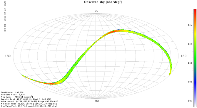
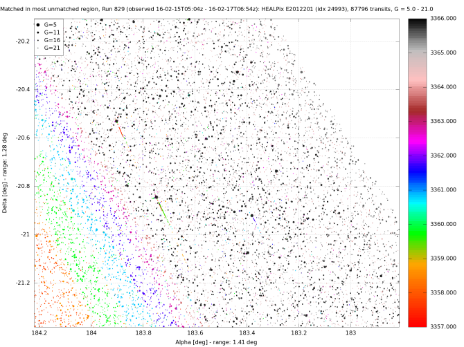
Figure 2.21: Example of sky region diagnostics in IDT, with a Mollweide projection of the density of transits processed during the last few hours (top panel, in transits per square degree, in equatorial coordinates), and a sky chart with the detections, times (in colour) and brightness (in the size of the dots) observed around a specific region (bottom panel). -
–
-
•
Photometric features (Figure 2.22):
-
–
Distribution of the number of transits per magnitude, in the , , and bands.
-
–
‘Colour’ distribution, showing the transits per – pseudo-colour, per effective wavelength, etc. Also colour–colour plots are determined, showing the effective wavelength distribution per – colour.
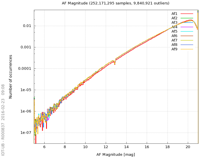
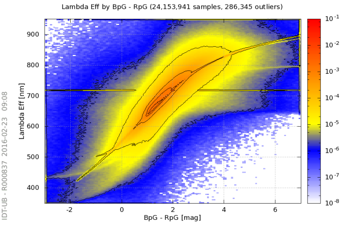
Figure 2.22: Example of transits density per -mag (left panel), which illustrates the exponential increase in star density with magnitude. The 2D histogram in right panel illustrates the correlation between some of the preliminary colour features found by IDT, namely, the effective wavelength (which in turn correlates with the star temperature) and a colour index (based on the magnitude difference between and bands). -
–
-
•
Attitude diagnostics (Figure 2.23, Figure 2.24 and Figure 2.25):
-
–
Distribution of match distances between the detections used by OGA1 and their associated sources.
-
–
Average number of detections per second used in OGA1 attitude reconstruction.
-
–
Time series with the difference, in field angles (along and across scan), between the reconstructed attitude (OGA1) and the raw or IOGA attitudes. Also time series with the attitude rates (along and across scan) are determined.
-
–
Motions estimated for the transits processed, determined from the AF observation times and the attitude rates.
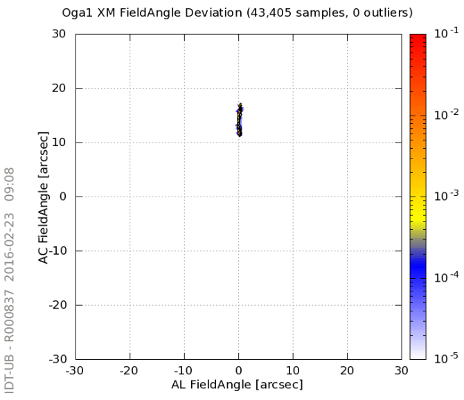
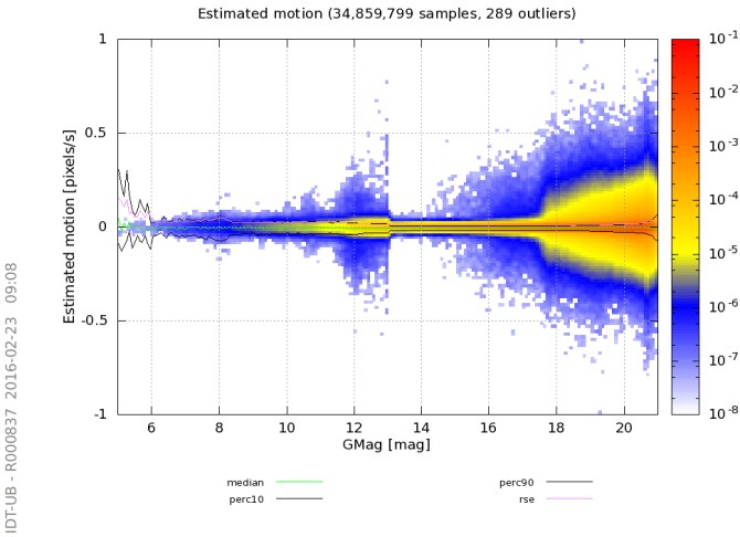
Figure 2.23: Left panel shows a distribution of match distances (in field angles) between the detections used in OGA1 and their associated stars. Right panel shows some results of the motions estimated for transits processed by IDT (in pixels per second, where 1 pix/sec means 60 mas/sec) as a function of the -mag estimated on-board. 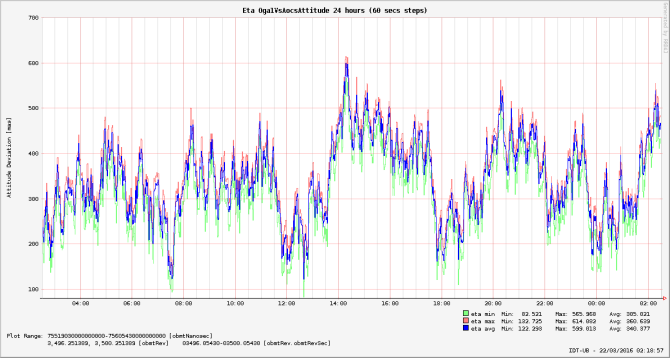
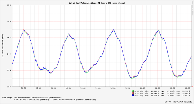
Figure 2.24: Difference between the first on-ground attitude refinement (OGA1) and the raw attitude determined on-board, which can be seen as the correction to be applied to such raw attitude. It is shown for the along-scan field angle (left panel) and one of the across-scan angles (right panel). The 6-hours periodicity is due to small variations in the alignment between the star tracker and the payload module. 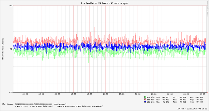
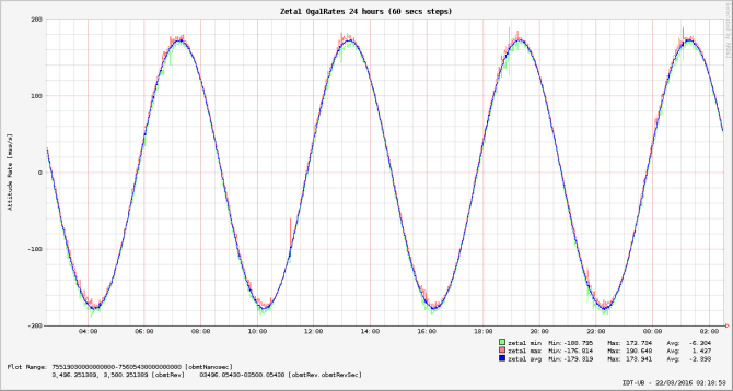
Figure 2.25: Along scan (left panel) and across scan (right panel) rates determined from OGA1. Along-scan rates help identifying small micro meteoroid impacts on the spacecraft. Across-scan variations are caused by precession. -
–
-
•
Bias diagnostics (Figure 2.26):
-
–
Histograms with the distribution of Bias and Read-Out Noise (RON) values per CCD.
Figure 2.26: Snapshot of an IDT WebMon page showing the readout noise levels per CCD (larger). -
–
-
•
Background diagnostics (Figure 2.27):
-
–
Histograms with the astrophysical background level (in electrons per pixel per second) determined per CCD.
Figure 2.27: Snapshot of an IDT WebMon page showing the astrophysical background levels determined per CCD, where we can see the higher levels for some CCDs due to stray light (larger). -
–
-
•
Image parameters diagnostics (Figure 2.28):
-
–
Outcome of the Image Parameters Determination (IPD), indicating the fraction of windows with problems in the fitting.
-
–
Distribution of the ‘centroiding’ (astronomical IPD) position within the SM or AF window, revealing possible problems in the on-board centring of the windows or in the PSF/LSF calibration.
-
–
Goodness-of-fit distribution, based on a estimation.
-
–
Distribution of formal errors in the fitting, as provided by the algorithm in itself.
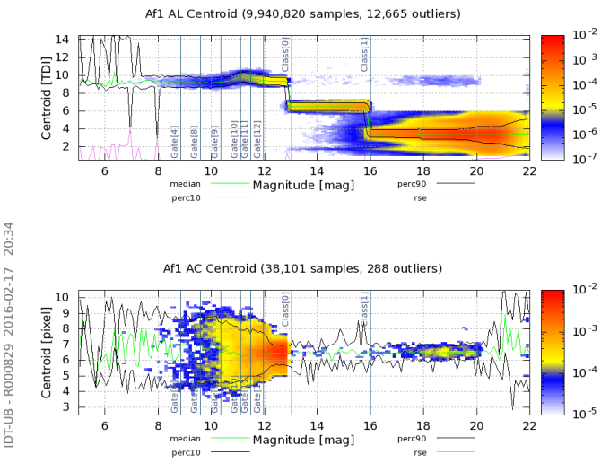
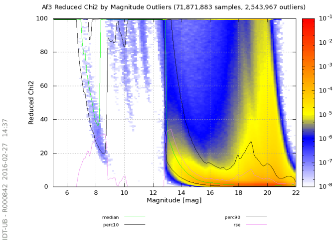
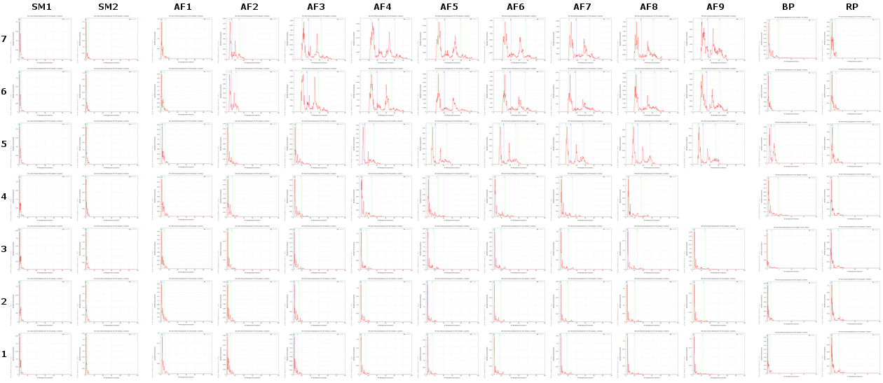
Figure 2.28: Left panel: example of the centroids distribution determined for a given CCD (AF1 in this case), along and across scan within the acquisition window, as a function of the on-board magnitude estimation. It illustrates the different sampling scheme depending on the brightness. Right panel: goodness-of-fit in the astrometric image parameters determination, which shows reasonable fits for 1D windows (faint detections) and much worse for bright detections (due to the simplistic 1D1D PSF model used in IDT). -
–
-
•
Crossmatching diagnostics (Figure 2.29):
-
–
Number of matched and unmatched transits (that is, detections for which no source has been found in the catalogue at a distance closer than 1.5 arcsec), number of detections identified as ‘spurious’, and number of new source entries created.
-
–
Distribution of match distances in the along and across scan directions.
-
–
Ambiguity in the crossmatch solution, indicating the fraction of transits for which more than one candidate source was found.
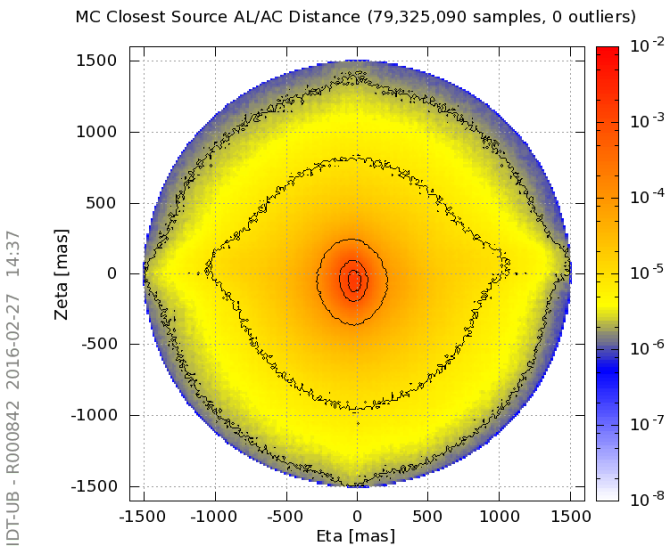
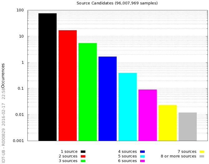
Figure 2.29: Left panel: distribution (in field angles) of the match distance in the daily crossmatch, revealing some features due to on-board spurious detections. Right panel: ambiguity in the crossmatch solution from IDT. -
–
First-Look diagnostics (FL)
Astrometric space missions like Gaia have to simultaneously determine a tremendous number of parameters concerning astrometry and other stellar properties, the satellite’s attitude as well as the geometric, photometric, and spectroscopic calibration of the instrument.
To reach inherent level of precision for Gaia, many months of observational data have to be incorporated in a global, coherent, and interleaved data reduction. Neither the instrument nor the data health can be verified at the desired level of precision by standard procedures applied to typical space missions. Obviously it is undesirable not to know the measurement precision and instrument stability until more than half a year of the mission has elapsed. If any unperceived, subtle effect would arise during that time this would affect all data and could result in a loss of many months of data.
For this reason a rapid ‘First Look’ was installed to daily judge the level of precision of the (astrometric, photometric and spectroscopic) stellar, attitude and instrument calibration parameters and to achieve its targeted level by means of sophisticated monitoring and evaluating of the observational data. These daily checks include analyses of
-
•
astrometric science data with the help of the so-called One-Day Astrometric Solution (ODAS) which allows to derive an accurate on-ground attitude, improved source parameters, daily geometric instrument parameters as well as astrometric residuals required to assess the quality of the daily astrometric solution,
-
•
photometric and spectroscopic science data in order to assess the CCD health and the sanity of the LSF/PSF and spectroscopic calibrations,
-
•
the basic-angle monitor (BAM) data which aims at independently checking the behaviour of the Gaia basic angle,
-
•
auxiliary data such as on-board data needed to allow for a proper science data reduction on ground and on-board processing counters which allow to check the sanity of the on-board processing, and
-
•
the satellite housekeeping data.
The First Look aims at a quick discovery of delicate changes in the spacecraft and payload performance, but also aims at identifying oddities and proposing potential improvements in the initial steps of the on-ground data reduction. Its main goal is to influence the mission operations if need arises. The regular products and activities of the First-Look system and team include:
-
•
The so-called One-Day Astrometric Solution (ODAS) which allows to derive a high-precision on-ground attitude, high-precision star positions, and a very detailed daily geometric calibration of the astrometric instrument. The ODAS is by far the most complex part of the First-Look system.
-
•
Astrometric residuals of the individual ODAS measurements, required to assess the quality of the measurements and of the daily astrometric solution.
-
•
An automatically generated daily report of typically more than 3000 pages, containing thousands of histograms, time evolution plots, number statistics, calibration parameters etc.
-
•
A daily manual assessment of this report. This is made possible in about 1–2 hours by an intelligent hierarchical structure, extended internal cross-referencing and automatic signalling of apparently deviant aspects.
-
•
Condensed weekly reports on all findings of potential problems and oddities. These are compiled manually by the so-called First Look Scientists team and the wider Payload Experts Group (about two dozen people). If needed, these groups also prompt actions to improve the performance of Gaia and of the data processing on ground. Such actions may include telescope refocusing, change of on-board calibrations and configuration tables, decontamination campaigns, improvements of the IDT configuration parameters, and many others.
-
•
Manual qualification of all First-Look data products used in downstream data processing (attitude, source parameters, geometric instrument calibration parameters).
In this way the First Look ensures that Gaia achieves the targeted data quality, and also supports the cyclic processing systems by providing calibration data. In particular the daily attitude and star positions are used for the wavelength calibration of the photometric and spectroscopic instruments of Gaia. In addition, the manual qualification of First-Look products helps both IDT and the cyclic processing teams to identify and discriminate healthy and (partly) corrupt data ranges and calibrations. This way, bad data ranges can either be omitted or subjected to special treatment (incl. possibly a complete reprocessing) at an early stage.
Astrometric Instrument Model (AIM) diagnostics
The main objective of the AIM system is the independent verification of selected AF monitoring and diagnostics, of the image parameters determination, instrument modelling and calibration. It can be defined as a scaled-down counterpart of IDT (see Section 2.4.2) and FL (see Section 2.5.2) restricted to some astrometric elements of the daily processing, those which are particularly relevant for the astrometric error budget. This separate processing chain runs in Gaia DR1 with the following 6 modules: Astrometric Raw Data Processing, Selection, Monitoring, Daily Calibration, CalDiagnostic and Report; several CalDiagnostic tasks run also off-line. Each AIM processing steps can be divided into three main parts: input, processing and output steps.
Raw Data Processing
The main goal of the Raw Data Processing (RDP) is the determination of image parameters like AL and AC centroid, formal errors, flux and background. A high density region filter runs before starting RDP when the satellite scans the Galactic plane to process only the useful observations for the other AIM processing steps. The goal is to maintain the AIM capability to give a quick feedback on the astrometric instrument health and data reduction issues, if any.
-
1.
The RDP inputs are the raw data (see Section 2.2.2) and selected outputs of the IDT system, namely:
-
–
AstroObservation with window class 0 and 1, e.g. brighter than G16.
-
–
PhotoElementary
-
–
-
2.
The RDP outputs are the image parameters, i.e. centroid, formal errors, flux and local background stored within the AimElementaries. This allows routine comparisons with — and thus external verification of — IDT centroid values and corresponding formal errors. In addition to that there are also specific inputs for the Monitoring processing.
Selection
The module selects the good observations for performing daily calibration. Indeed, for image profile reconstruction only well-behaved observations must be selected, spread over the whole AIM Gmag range. This means far from a charge injection event (more than 30 TDI lines) and with good image parameters fit results.
-
1.
The Selection inputs are:
-
–
AstroObservation
-
–
PhotoElementary
-
–
AstroElementary
-
–
AimElementaries
-
–
-
2.
The Selection outputs are the SelectionItems.
Monitoring
Monitoring is a collection of software modules, each dedicated to perform a particular task on selected data sets with the goal to extract information about instrument health, Astro instrument calibration parameters and image quality during in-flight operations over a few transits or much longer time scales.
-
1.
The Monitoring inputs are:
-
–
AimElementaries
-
–
MonitorDiagnOutputs
-
–
AstroObservation and AstroElementary
-
–
-
2.
The Monitoring outputs are plots and statistics among which:
-
–
AIM centroid
-
–
Formal errors AC and AL vs. Gmag for each CCD
-
–
AIM centroid residual variation AL and AC vs. Gmag for each CCD
-
–
AIM centroid residual variation AL and AC vs. time for each CCD
-
–
AIM Image moments distribution over each row for each spectral bin
-
–
Detections number for each magnitude and wavelength bin
-
–
AIM AC and AL centroid mean variation over the row for each wavelength bin
-
–
AIM AC and AL centroid mean variation over time and wavelength vs. strips
-
–
Comparison among AIM and IDT centroid
-
–
Formal errors
-
–
Daily Calibration
Two of the Gaia key calibrations are the reconstruction of the Line and Point Spread Functions. For that reason AIM implements its own independent Gaia signal profile reconstruction on a daily basis. The PSF/LSF image profiles model is based, in a one dimensional case, on a set of monochromatic basis functions, where the zero-order base is the sinc function squared, which depends on an a-dimensional argument , related to the focal plane coordinate , the wavelength , and the along-scan aperture width of the primary mirror. This corresponds to the signal generated by a rectangular infinite slit of size , in the ideal (aberration-free) case of a telescope with effective focal length (see Equation 2.46).
| (2.46) |
The contribution of finite pixel size, Modulation Transfer Function (MTF) and CCD operation in time-delay integration (TDI) mode are also included. The higher-order functions are generated by suitable combinations of the parent function and its derivatives according to a construction rule ensuring orthonormality by integration over the domain. The polychromatic functions are built according to linear superposition of the monochromatic counterparts, weighted by the normalized detected source spectrum which includes the response of the system.
The spatially variable LSF/PSF is reconstructed as the sum of spatially invariant functions, with coefficients varying over the field to describe the instrument response variation for sources of a given spectral distribution. We then fine tune the function basis to the actual characteristics of the signal by using a weighting function built from suitable data samples (Gai et al. 2013)). The profile reconstruction is obtained using at most 11 terms for 1D profiles and between 30 and 65 terms for full 2D windows. Only the 1D profile reconstruction ran during the time interval covered by the Gaia DR1. The upper limit of the astrometric error introduced by the fitting process for the 1D reconstruction is less than pixels, while the photometric error in is less than .
The ’astrometric error’ is the systematic error in the image position determination and the ’photometric error’ is the flux loss or flux gain using the selected model for the image flux determination. They are injected as a residual by the fit process which aims at reconstructing the image profile by building the template for the selected data set.
Our modelling is based on only 11 ad-hoc base functions derived from a physical (simplified) representation of the opto-electronic system. The base functions depend on just two tuning parameters, therefore we need to check that the model is robust, and the right solution for each template unit is chosen as the one which introduces a negligible ’astrometric’ bias, i.e. a negligible error on the position determination. It may be taken as the residual mismatch between the data set and its fit. They are not the astrometric and photometric error on the elementary exposure or on the Gaia final accuracy. If we want to reach a final accuracy of 10 and m-mag level we need of course to have the systematic errors one order smaller at most. The good solution for each bin (the LSF template for that bin) is the one that introduces an ’astrometric’ error and a ’photometric’ error below a given threshold. All the templates realize the LSFs library.
An AIM LSF/PSF library contains a calibration for each combination of telescope, CCD, source colour (wavelength for Gaia DR1) and AC motion. The LSF/PSF calibration will improve during the mission with each processing calibration cycle outputs.
-
1.
The Daily Calibration inputs are:
-
–
AimElementaries
-
–
SelectionItems
-
–
MonitDiagnosticOutputs
-
–
LsfsForLasAL
-
–
LsfsForLasAC
-
–
AstroElementary
-
–
CalibrationFeatures
-
–
-
2.
The Daily Calibration outputs are the results of the fitting procedure:
-
–
CalModulesResultsAL and CalModulesResultsAC
-
–
CcdCalFlag
-
–
The LSFs library InstrImageFitLibrariesAL and InstrImageFitLibrariesAC.
-
–
CalDiagnostic
-
1.
The CalDiagnostic inputs are the outputs from the Daily Calibration
-
–
CalModulesResultsAL
-
–
CalModulesResultsAC
-
–
-
2.
The CalDiagnostic outputs are plots and statistics among which:
-
–
Focal plane average image quality variation for each AIM run which includes variation with colours over the row
-
–
Average colours variation over the row
-
–
Variation with colours over the strip
-
–
Average colours variation over the strip
-
–
Calibrated PSF template coefficient variation over the row depending on colours which includes template moments variation over the row depending on colours
-
–
Template moments variation over the row averaged over colours
-
–
There are also a few tasks which perform trend analyses of the PSF/LSF image moments variations over weekly, monthly and/or longer interval times which can be selected by the operators in near real time.
The AIM system has also an internal automatic validation/qualification of the processing steps results, but manual inspection is needed for some particular outputs as, for example, the outputs coming from the comparison tasks with the main pipeline outputs.
Each day a report is automatically produced collecting plots and statistics about RDP, Calibration, instrument health monitoring and diagnostics. The daily reports are thousands pages and only for internal use. When needed, a condensed report about the findings of potential problems is reported to the Payload Experts group. This way, the AIM team supports the DPAC cyclic processing systems by guaranteeing a high quality level of the science data. No data produced by the Astrometric Instrument Model software enters the first Gaia data release.
Basic Angle Monitoring (BAM) diagnostics
The BAM instrument is basically an interferometer devoted to the monitoring of the Lines-Of-Sight (LOS) of each telescope. The instrument measures and monitors the variation of the Base Angle value between the two telescopes looking at the phase changes of the fringes.
The AVU/BAM system monitors on a daily basis the BAM instrument and the basic angle variation (BAV) independently from IDT (see Section 2.4.2) and FL (see Section 2.5.2), to provide periodic and trend analysis on short and long time scales, and to finally provide calibrated BAV measurements, as well as a model of the temporal variations of the basic angle.
It is a fundamental component of the technical and scientific verification of the overall Gaia astrometric data processing, and is developed within the context of the Astrometric Verification Unit (AVU). Deployment and execution of the operational system is done at the Torino DPC which constitutes one of six DPCs within the Gaia DPAC.
The input data to AVU/BAM (coming from DPCE) correspond to a central region of the fringe envelope for each line of sight. For Release Gaia DR1 the central region corresponds to a matrix of 1000 x 80 samples (ALong x ACross scan). Each of the 80 AC samples is onboard binned (4 physical pixel each sample). BAM CCDs are the same kind of RP CCDs, and have a pixel size of 10 by 30 , (AL x AC).
The system, besides producing the fundamental BAM measurements (e.g. time series of the phase variation), processes the elementary signal and provides an interpretation in terms of a physical model, to allow early detection of unexpected behaviour of the system (e.g. trends and other systematic effects). An important function performed by the BAM is to provide ways to identify and quantify the underlying causes in case the specific passive stability of the basic angle should be violated in orbit. The AVU/BAM pipeline performs two different kinds of analyses: the first is based on daily runs, the second is focused on overall statistics on a weekly/monthly basis.
The most important output is the Basic Angle Variation (BAV) estimate. In principle it is the differential variation of the two LOS. The pipeline provides the BAV estimate through three different algorithms ]2014RMxAC..45…35R.
The first one, named Raw Data Processing (RDP) (similar to the IDT approach), provides the BAV as a difference of the variation of the two LOS. Each LOS estimate is performed through a cross correlation of each BAM image with a template made by the mean of first 100 images of each run. The second algorithm, named Gaiometro, is the 1D direct cross correlation between the two LOS. The third one is a 2D version of the direct measurement of BAV Gaiometro 2D. Indeed the first two use images binned across scan.
The four independent results (three AVU/BAM plus IDT) agree quite well in the general character and shape of the 6-hour basic-angle oscillations, while the derived amplitudes differ at the level of 5 percent. It is as yet unknown which of the four methods (and of the implied detailed signal models fitted to the BAM fringe patterns) gives the most faithful representation of the relevant variations in the basic angle of the astrometric instrument.
In addition to producing time series of the fringe phase variations, AVU/BAM also makes measurements of other basic quantities characteristic of the BAM instrument, like fringe period, fringe flux and fringe contrast. Their temporal variations are also monitored and analysed to support the BAV interpretation.
The Fringe Flux is calculated as the raw pixel sum of each frame. The second one is the Fringe Period , that is given by
| (2.47) |
with, is the focal length, is the wavelength and is the baseline. This quantity gives a fast overlook to these three properties of the BAM instrument. The Fringe Contrast is basically related to the visibility of the fringes.
AVU/BAM provides also an independent calibration of quantities like BAV. An initial internal calibration of BAV measurements has been activated since December 2014.
AVU/BAM crew produces a periodic report with a summary of the evaluated quantities and the events found in each time interval. Most important events are directly (manually) checked with FL scientists and Payload Experts groups.
The AVU/BAM outputs are made available to the other relevant DUs in CU3 (AGIS, GSR, FL). No data produced by the AVU/BAM software enters the first Gaia data release.
2.5.3 Monitoring of cyclic pre-processing
Author(s): Javier Castañeda
The cyclic pre-processing scientific performance is assured by specific test campaigns carried out regularly by the DPCB team in close collaboration with all the IDU contributors. For these tests, detailed analysis over the obtained results are done — even including the execution of reduced iterations with other systems.
As already commented in previous sections, IDU processes a huge amount of data and produces similarly a huge amount of output. The continuous and progressive check on the quality of these results is not a desirable feature. The analysis of every calibration and parameter produced by IDU (as it is done for the test campaigns) is not practically possible — it would have almost the same computational cost as the processing itself. For this reason, IDU integrates a modular system able to assure the quality of the results up to a reasonable limit.
First of all, IDU tasks includes several built-in consistency checks over the input and output data. These are really basic checks for:
-
•
verifying the consistency of the configuration parameters including their tracking along the full processing pipeline.
-
•
verifying the consistency of the input data, so corrupted data or inconsistent input data combinations do not enter the pipeline and are not propagated to subsequent tasks.
-
•
accounting for the number of outputs with respect to the inputs, so data lost is detected and properly handled – in general forcing a task failure.
Additionally, all IDU tasks integrate a validation and monitoring framework providing several tools for the generation of statistical plots of different kinds. This framework provides:
- Bar Histograms
-
Histograms for the characterisation of the frequency of parameters with limited number of values.
For example the processing outcome of the image parameter processing, counts of observations per row, etc. - 1D Histograms
-
Histograms for the computation of the frequency of non discrete parameters; including the computation of statistical parameters as mean, variance and percentiles.
- 2D Histograms
-
Histograms showing the distribution of values in a data set across the range of two parameters. They support static dimensions or abscissae dynamic allocation. The first type is mainly used for the analysis of 2D dependencies or 2D density distributions of two given parameters — usually the abscissae parameter is the magnitude whereas the second type is used for analysis of the evolution of a given parameter as a function of a non restricted increasing parameter — typically the observation time. The bins can be normalised globally or locally for each abscissae bin. Percentiles as well as contours are also supported.
- Sky Maps
-
Plots generated from a histogram based in the HEALPix Górski et al. (2005) tessellation and implementing the Hammer-Aitoff equal-area projection. The plots can represent the pixel count, pixel density or the pixel mean value for a given measured parameter. Mainly used to obtain the sky distribution of some particular object (sources, observations, etc.) or to analyse the alpha and delta dependency of some parameter mean value, i.e. the astrophysical background, proper motion, etc.
- Sky Region Maps
-
Tool for plotting sources and detections in small ICRS-based sky regions. Mainly used for the analysis of the crossmatch and detection classification results.
- Focal Plane Region Maps
-
For the representation of the observations according to their along and across focal plane coordinates. Mainly used for the analysis of the scene and detection classification results.
- Round-Robin Database (RRD)
-
Round-Robin Databases are typically used to handle and plot time-series data like network bandwidth, temperatures, CPU load, etc. but they can also be use to handle other measurements such as the quaternion evolution, observation density, match distance evolution, etc.
- Range Validators
-
Implement very basic field range validation against the expected nominal parameter values.
- TableStats
-
Collector of statistics for miscellaneous table fields. Basically provides counters for the discrete values of predefined fields or for boolean flags/fields.
All Histograms and the Sky Maps, share a common framework allowing the split of the collected statistical data according to the FoV, CCD row, CCD strip, window class, source type, etc. This functionality is very useful for restricting the origin of any feature visible in the global plots — in that sense the user can see if some plot peculiarity or feature are present only in one of the FoV, rows or for a given source type and detect possible problems in the calibrations.
All these tools are also integrated in daily pipeline and they are used for its monitoring on a daily basis. A handful of examples of the plots obtained using these tools have been included in Section 2.5.2, Section 2.4.9 and Section 2.4.9.
All these tools ease the monitoring of the cyclic scientific results but unfortunately they are not enough to guarantee the quality of the outputs. Specific diagnostics are needed to also assure the progressive improvement with respect to the results obtained in previous iterations. Some examples of these diagnostics are:
-
•
For all tasks in general:
-
–
Range validation against expected nominal parameters.
-
–
-
•
For the crossmatch and detection classification tasks:
-
–
Monitoring of the amount of new sources created compared with previous executions.
-
–
Monitoring of the time evolution of the along and across distance to the primary matched source obtained in the crossmatch.
-
–
Check the evolution of matches to a predefined set of reference sources, to check if the overall transits have been assigned differently now, as compared to the previous cycle.
-
–
Monitoring of the evolution of the number of spurious detection density for very bright sources.
-
–
-
•
For the image parameters:
-
–
Monitoring on the goodness-of-fit of the LSF/PSF fitting obtained.
-
–
Comparison of the derived image parameters against the astrometric solution over a pre-selection of well-behaved sources.
-
–
Cross-check of the residuals from the previous statistic against the chromatic calibration residuals from the astrometric solution.
-
–
Additionally, it is worth pointing out that the computational performance and the correct progress of the processing is also monitored. IDU integrates different tasks, presenting different I/O and computational requirements. A good balancing of the task jobs is essential to exploit the computational resources and to be able to meet the wall clock constraints of the data reduction schedule. This balancing is only feasible when we have a good knowledge of the processing performance profile of each task in terms of CPU time, memory and I/O load.
These performance metrics are a built-in feature of IDU framework. Each task provide measurements for:
-
•
Number of elements processed: sources, observations, time intervals, etc.
-
•
Total time elapsed for data loading, data writing and for each data processing algorithm.
-
•
File system timing on file access, copy and deletion.
-
•
Total CPU and I/O time accounted for each processing thread.
With all this information several diagnostics are generated to obtain the scalability of each task to different parameters. These diagnostics provide very valuable information on how the tasks scale when the data inputs are increased; i.e. linearly or exponentially. These plots are obtained by executing each task in isolation with different configurations, mainly covering larger time intervals or sky regions.
Besides this overall task profiling, more detailed information can also be obtained for the profiling of some specific parts of the processing. These diagnostics are very useful to detect possible bottlenecks or unexpected performance degradation for specific parts of the processing or for specific data chunks.
Please note that for Gaia DR1 only the scene, detection classification and crossmatch diagnostics apply.